Architecture

SpectraFuse has two pipelines. Ingestion (SpectRAGIngestion) runs once per document set and saves an index folder. Retrieval (SpectRAGRetrieval) loads that folder and runs once per question.

Interactive walkthrough: click through all ten stages on a 12-chunk corpus, inspect any chunk or edge, and move the selection sliders. Open it in a full window.

The problem it solves

Take the question "Which city is the headquarters of the lab that does the research for Project Orion?" Two chunks answer it together:

• c4, in the Project Orion document: "The research work for Project Orion is carried out by Helix Labs."
• c6, in the Helix Labs document: "Helix Labs is headquartered in Pune."

c6 never mentions Project Orion. In the walkthrough corpus, dense similarity ranks it 6th of 12, behind three near-identical "Project Orion research targets…" chunks. A top-k retriever with a 70-token budget fits only its first five chunks, so c6 never reaches the LLM.

SpectraFuse links c4 and c6 through the entity Helix Labs. It reaches c6 by walking the graph, then prefers it over a fourth Orion chunk because it opens a new document and a new community, and repeats nothing already chosen.

Offline: ingestion

SpectRAGIngestion("my_index", settings).ingest("docs/")

Step	What happens	Paper	Module
1. Load	Read .txt, .md and .pdf files; each file is one document		utils/loader.py
2. Chunk	Split by headings, keeping each chunk's section path, or where the topic changes (90th-percentile sentence distance). At most chunk_tokens (1,200) tokens with overlap_tokens (100) overlap; sentences and table rows are never cut	Section 3.3	utils/chunker.py, utils/sections.py, utils/semantic_split.py
3. Annotate	Entities (rule-based, or your entity_fn), references to sections and files, and utility questions (with your question_fn)	Section 3.2.1	utils/entities.py, utils/references.py, utils/questions.py
4. Embed	nomic-embed-text with the search_document: prefix, the offline hash embedder, or your function; vectors are L2-normalised	Table 1	utils/embedder.py, utils/vector_index.py
5. Edge signals	Six links between chunks, each in [0, 1]	Section 3.2.1	utils/edges*.py
6. Weighted graph	Weighted sum of the signals; edges below τ dropped; each chunk keeps its graph_k strongest edges	Eq. 10	utils/graph_build.py
7. Spectral coordinates	The smallest non-trivial eigenvectors of the normalised Laplacian: 32 numbers per chunk that say where it sits in the graph	Eq. 11–13	utils/spectral.py
8. Clusters	k-means on the row-normalised coordinates, for the selector's coverage term	Section 3.4	utils/clusters.py
9. Save	Binary arrays and JSON files, written to <folder>.partial and moved into place when complete	Table 1	utils/store.py

The six edge signals

Signal	Links two chunks when they...	Default weight α
semantic	are among each other's semantic_k (10) nearest neighbours by embedding (either direction); weight = cosine	0.300
section	are in the same section of a document (1.0), or in sibling or parent and child sections (shared headings ÷ longest path)	0.250
entity	mention the same entities (Jaccard overlap of their entity sets)	0.200
adjacency	are next to each other in the same document	0.084
utility	can answer similar questions (cosine of their utility-question embeddings, k nearest neighbours)	0.083
citation	one refers to the other: a numbered section (Section 2.1, §4) or another document by file name (notes.md)	0.083

The weights are the paper's signal configuration 1. A signal with no edges in your corpus (for example utility, when no question_fn is given) gives its weight to the others, in proportion.

\[ w_{ij} = \sum_{r} \alpha_r \, w^{(r)}_{ij}, \qquad \text{keep the edge if } w_{ij} \ge \tau \]

Spectral coordinates

From the weight matrix \(W\) and the degrees \(D\), the normalised Laplacian is

\[ L_{sym} = I - D^{-1/2} \, W \, D^{-1/2} \]

Its eigenvectors \(u_2, \dots, u_{33}\) (the first is trivial) give each chunk a 32-number coordinate \(z_i\). Chunks that are strongly linked get similar coordinates, so communities of the corpus become clusters of points. The spectral part explains why.

Online: retrieval

result = SpectRAGRetrieval("my_index").search(question, token_budget=4000)

A three-hop question on the 14-document example set: seeds, the two-hop walk, PageRank scores, and the 256-token budget. This example was chosen to show the mechanism (64-token chunks, 3 edges per chunk, 2 seeds); measured results are in Benchmarks.

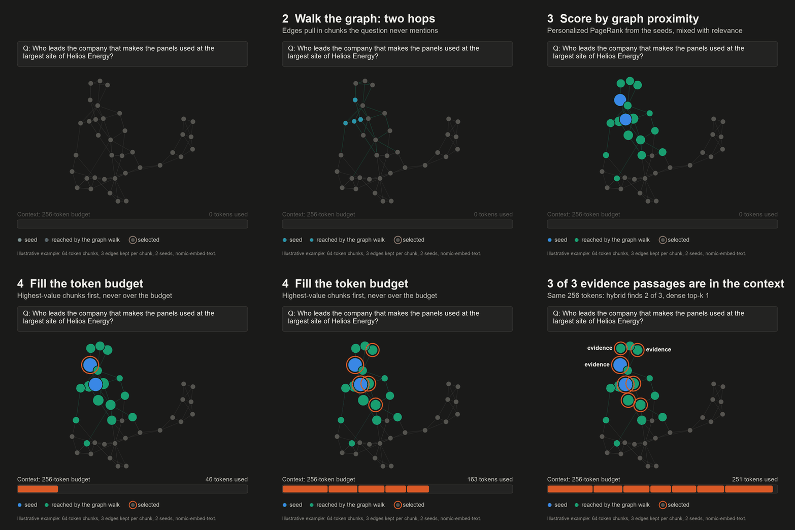
Step	What happens	Paper	Module
1. Hybrid seeds	Dense, BM25 and utility-question rankings fused with reciprocal rank fusion → seed_count (20) seeds, and a relevance score for every chunk	Table 2	utils/seeding.py, utils/bm25.py
2. Graph expansion	Breadth-first search from the seeds, hops (2) hops, at most max_candidates (200) chunks: this is where bridge evidence enters	Section 3.6	utils/expansion.py
3. Proximity re-scoring	Relevance blended with graph proximity: Personalized PageRank from the seeds and spectral closeness	Eq. 17–18	utils/diffusion.py
4. Token-budget selection	A protected core, a greedy tail that trades relevance against redundancy, coverage and length, then backfill; never over the budget	Eq. 19–22	utils/selection.py, utils/selectors.py
5. Context and answer	Selected chunks grouped by document, in a grounded prompt for any LLM	Algorithm 1	utils/prompt.py, utils/llm.py

Seeds

\[ \mathrm{RRF}(c) = \sum_{\text{lists}} \frac{1}{k + \mathrm{rank}(c)}, \qquad k = 60 \]

The relevance of a chunk is \((1 - w)\cdot\text{dense} + w\cdot\text{BM25}\), both scaled to 0…1, with \(w\) = bm25_weight (0.5).

Re-scoring

Personalized PageRank spreads the seeds' relevance over the candidate subgraph (\(\tilde{A} = D^{-1/2} W D^{-1/2}\), restart share \(\beta\) = ppr_beta, 0.15):

\[ s^{(t+1)} = \beta \, r + (1-\beta)\, \tilde{A}\, s^{(t)} \]

The default proximity_mode = "hybrid" averages it with spectral closeness to the seeds, then

\[ \text{score}(c) = (1-\alpha)\,\text{relevance}(c) + \alpha\,\text{proximity}(c), \qquad \alpha = 0.3 \]

Selection

The selector first keeps the core_size (3) best-scored chunks. It then repeatedly adds the chunk with the best utility per token, among chunks above the precision floor:

\[ U(c \mid C) = a\, s_c + b\,\text{Prox}(c) + c\,\text{ClusterGain}(c, C) + d\,\text{DocGain}(c, C) - \lambda\,\text{Red}(c, C) \]

\[ c^{*} = \arg\max_{c} \frac{U(c \mid C)}{\ell(c)^{\rho}}, \qquad \sum_{c \in C} \ell(c) \le B \]

• ClusterGain and DocGain are 1 for a chunk from a spectral cluster (or document) not yet in the context, ½ for the second, and so on: they reward coverage.
• Red is the highest cosine similarity to a chunk already chosen: it penalises near-duplicates.
• \(\ell(c)\) is the chunk's length in tokens and \(\rho\) = length_power (0.5).

Finally, backfill adds the best remaining chunks that still fit, so no budget is wasted. Other selectors (mmr, protected_mmr, anchor_expand_ce, topk) are described in Configuration.

Design decisions

The paper leaves some details open: for example the value of \(\rho\), the edge threshold \(\tau\), and how entities are found. Every such choice, and why it was made, is listed in DESIGN.md (decisions D1–D64).